Imagine a production line in which only good parts are produced (100% quality), as fast as possible (100% performance) and without stops (100% availability). The Overall Equipment Effectiveness (OEE) would equal 100%, which means “perfect production”. Even though dreams can come true (100% OEE), perfect production is rather rare, and in many cases, the manufacturing shop-floor can become, for those directly involved in the production, a nightmare instead. Machines fail for several reasons, humans make mistakes and all of this together makes it impossible to achieve perfection.
The good news is that there is always room for improvement, i.e. we can always do things better. Aiming at that, a continuous improvement process should be put in place to tackle exactly what prevents a production line from being perfect. In the “Theory of Constraints”, Eliyahu M. Goldratt, author of the best-selling book titled “The Goal”, argues that one should follow “The Five Steps of Focusing” to achieve the goal (e.g. maximize overall throughput):
- Identify the system’s constraint(s);
- Decide how to exploit the system’s constraint(s);
- Subordinate everything else to the above decision(s);
- Alleviate the system’s constraint(s);
- If in the previous steps a constraint has been broken, go back to step one (i.e. repeat as needed).
The above mentioned theory states that “the throughput of any system is determined by one constraint”. Let’s thus start from the beginning and focus on how to identify this constraint, or in other words “the bottleneck”.
Start from the beginning
Consider a production line as illustrated in Fig. 1. It consists of four machines and three buffers or accumulators (finite buffers, i.e. they can store only a finite amount of parts). Discrete parts flow from M1 to M4 and visit all machines and buffers in a fixed sequence, or in other words, each machine feeds only one buffer and each buffer feeds a single machine. Non-conformities or scrap can leave the line after being processed at every single machine. The net production for a specific period of time equals the number of parts entering the first machine (gross production) minus the sum of scrap produced in the line.
This type of production line depicted in Fig. 1 is known as the “asynchronous system”. The machines are, to a certain extent, decoupled from each other due to intermediate buffers. Thus, each machine can start and stop independently (asynchrony), even if they have exactly the same cycle time, provided that the neighbor buffers are neither empty nor full. Since the machines are not totally decoupled from each other, they can be blocked or starved. A machine is blocked if it is operational but the downstream buffer is full, which means no more parts can be stored on it and the machine is forced to stop (idle).
On the other hand, a machine is starved, if it is operational but the upstream buffer is empty, i.e. there are no parts available to be processed and the machine stops (idle). To illustrate this dynamic, Fig. 2 presents a simplified example of machine status, let’s assume it is M2 from Fig. 1, and the storage level of its neighbor buffers in a timeline containing six “time-steps” enumerated from 0 to 6. At time-step 0, M2 is active and the buffers are neither empty not full. After a while, the storage level of B1-2 starts decreasing, probably because M1 stopped due to a failure until it is completely empty at time-step 1.
At this moment M2 is starved and stops processing parts. At time-step 2, M2 starts processing parts again. A while after, B2-3 begins to fill up, probably because M3 or M4 stopped due to a failure, and gets completely full at time-step 3, where M2 is blocked. From time-step 4, M2 is active again until it stops at time-step 5. At this moment M2 is neither starved nor blocked, and thus it is in a failure-mode. B1-2 fills up and B2-3 empties. Fig. 2 thus illustrates a common dynamic that has to be followed to evaluate the status of every single machine in a production line.
Machine-status possibilities
In terms of availability, the following four machine-status are possible (three of them are illustrated in Fig. 2):
- Active: the machine is up and processing parts;
- Idle: the machine is either blocked or starved;
- Failure: the machine is down due to a failure;
- Stopped: the machine is down due to a planned activity, such as setups, planned maintenance, among others.
These four status set the basis and are crucial for identifying the bottleneck, but still some more information is required.
The reason for that is because an active machine can produce scrap and/or have longer cycle time when compared to other machines. Thus, availability, quality and productivity aspects have to be considered.
One possible solution is to adapt the OEE calculation. Instead of having an OEE for the entire production line, one has to adapt the calculation for every single machine. Let’s call it OEEbd, which stands for “OEE bottleneck-detection”. OEEbd differs from the usual OEE, because it does not consider idle-time as part of the available-time. Why not? The reason for that is because when a machine is idle, it is in this condition because it is restricted by another machine. Thus, only active-time and failure-time is considered as available time and is used to calculate OEEbd. At the end, the machine with the lowest OEEbd score at any given time instance is considered the bottleneck at that moment. It is important to mention this time-dependency, since bottlenecks can also shift from one machine to another due to different reasons.
Let’s check a simplified practical example, based on the production line depicted in Fig.1. We assume it is a packaging line, producing plastic tubes, at a maximal production rate of 250 tubes per minute. All machines have the same maximum speed, or in other words the same cycle-time. Data for thirty days of production is summarized in Table 1. The first five rows show the accumulated amount of days where each machine was active, blocked, starved, stopped or in failure-mode.
The gross production for the thirty days is 7 million tubes, that is the number of tubes that entered M1 (or were extruded). Net production and the correspondent
scrap rates are also presented in Table 1. The available time required to calculate OEEbd, as mentioned before, is the sum of active time and failure time. The ideal production is calculated based on the available time and would be the “perfect production” for this specific aggregated time. Since production rate is 250 tubes per minute (360,000 tubes per day), M1, for example, would have an ideal production of 8,280,000 tubes (23days multiplied by 360,000). Since M1 produced only 6,850,000 tubes, it’s OEEbd score is 82,7% (6,850,000 divided by 8,280,000). After repeating the same for all machines, one can see that M2 has the lowest OEEbd score (80,2%) and represents the bottleneck for this thirty days of production. Further interesting information can be seen from Table 1:
- Even though M1 and M2 have the same total failure time (3 days each), M2 has the lowest OEEbd score, since M2 has a higher scrap rate;
- Even though M3 spent one extra day in failure-mode when compared to M4, it has the highest OEEbd. The reason for that is because M4 has a scrap rate that is more than three times higher than M3’s scrap rate.
You should go a bit deeper: keep checking
In reality, the task of correctly assigning the different statuses to all machines is a great challenge. It cannot be solved through simple observation in fast production lines, as usual in the packaging industry. A big amount of data has to be collected, processed and analysed so that one can get the right insights. Sensors have to be strategically placed along the production line to gather all required information and a powerful algorithm has to run behind the scenes to solve this complex and important problem.
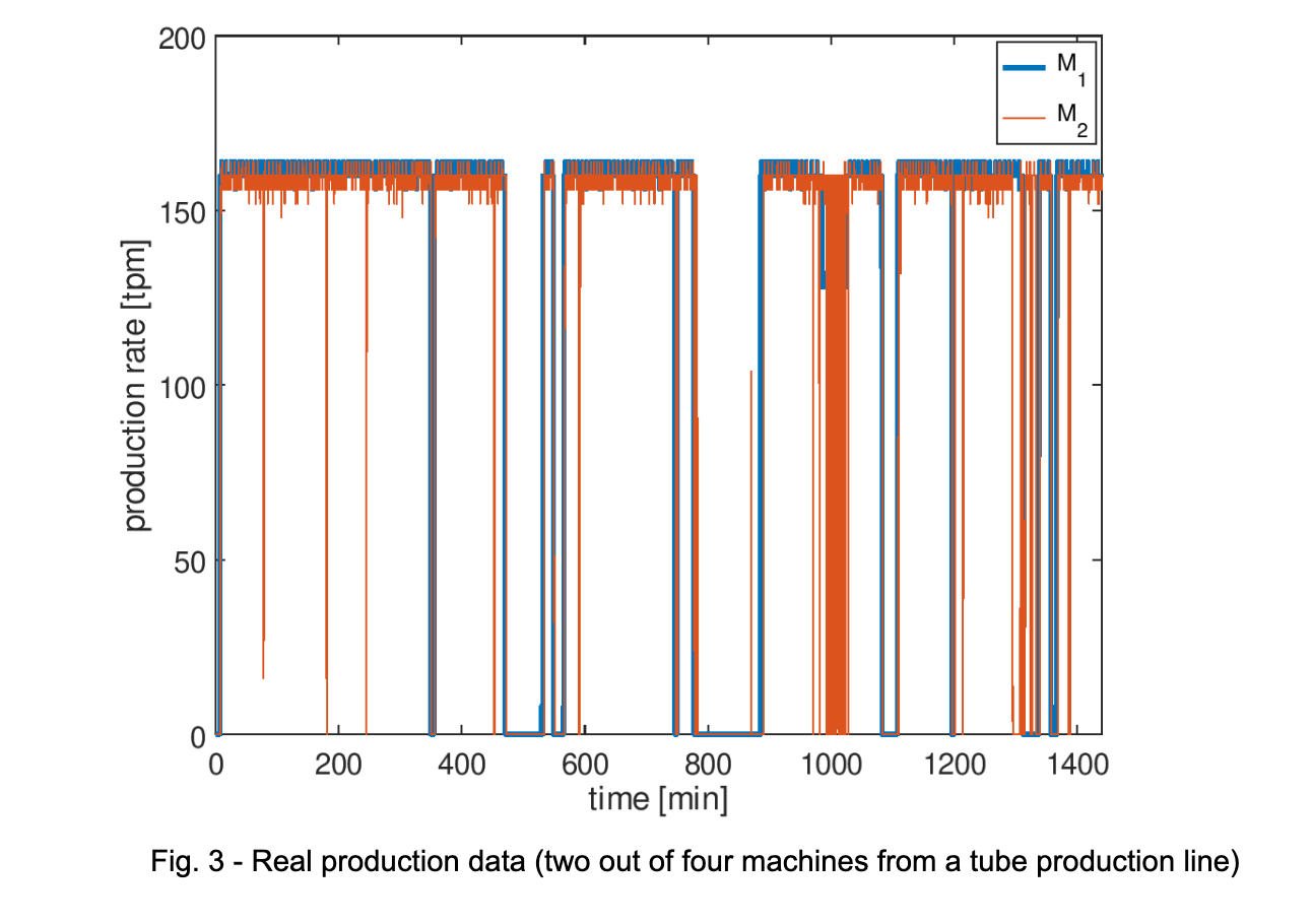
To illustrate this, Fig. 3 shows data from a real production line, in which only two machines are depicted for a 24-hours production. The production rate is 160 tubes per minute and one can see that both machines stop several times (micro-stops and long stops). Most of the time M1 restricts M2, so M2 starves because B1-2 gets empty. At around time 1,000 minutes, for example, M1 reduces production speed to 130 tubes per minute, causing M2 to have several micro-stops (B1-2 could not keep feeding enough parts to M2). Even though Fig. 3 can look relatively clear, adding more data, i.e. another few machines, accumulators, etc, would make complexity increase exponentially.
And what to do to overcome an identified bottleneck?
Now that the bottleneck has been detected in the previous example (Table 1), one should decide how to exploit it aiming at alleviating the constraint. The first hints from the table are “Failure Time” and “Scrap Rate”.
In the case of Failure Time, a more thorough assessment should be conducted to map the main causes of failures/downtime (fault diagnosis). Based on it, intermittent mechanical and/or electrical faults can be detected, so that a proper action plan can be set to mitigate their effects and increase the overall “Mean Time Between Failures”. Minimizing the “Mean Time to Repair” is also crucial.
This can be done by reducing the “Maintenance Response Time”, for example, by having automatic alarms notifying the maintenance team about faults. The maintenance team should also follow “Standard Maintenance Procedures” to guarantee minimal repair times. On top of that, a “Preventive Maintenance Plan” should be created focusing on the main detected failures. Capacity building and empowerment of operators/workers is another important strategy to run your factory more efficiently. Giving operators real-time information about what is going on on the shop floor can help them make quick decisions and consequently increase the overall efficiency of the production lines.
The above-mentioned strategies are just a few options to start the “battle”. Reminder: put a focus on quick wins to have immediate benefits. The main cause of equipment inefficiency is not necessarily the easiest to tackle. Start simple.
In terms of scrap, a very similar approach to what was mentioned above should be followed. Map it first. It can be a problem with the raw material, with inadequate adjustment/setup of the machine, with incorrect process parameters or even problems with the automated quality control systems, just to mention a few. So, quick wins first, and don’t forget to keep the operators informed in real time. They are always willing to have the best shift performance of the day/week, and you can help them by providing good quality information..
As the goal of any business is to make more money, a good start towards the goal is to identify the bottlenecks. Opportunities for improvement exist in every production line. Recognizing this fact and putting efforts to constantly find these opportunities is an important step to create a culture of continuous improvement in your organization.
Do you know where your bottlenecks are?
By Dr. Eduardo Weingärtner
Chief Data Officer – PackIOT
PhD from the Swiss Federal Institute of Technology Zurich (ETH)